- 🍨 本文为🔗365天深度学习训练营 中的学习记录博客
- 🍖 原作者:K同学啊 | 接辅导、项目定制
–来自百度网盘超级会员V5的分享
数据链接
提取码:7zt2
–来自百度网盘超级会员V5的分享
目录
- 0. 总结
- 1. 数据导入及处理部分
- 2. 划分数据集
- 3. 模型构建部分
- 3.1 调用官方的VGG16模型
- 3.2 自定义VGG16模型
- 3.3 公式推导
- 4. 设置超参数:定义损失函数,学习率,以及根据学习率定义优化器等
- 4.1 设置设置初始学习率,动态学习率,梯度下降优化器,损失函数
- 4.2 动态学习率代码说明
- 5. 编写训练函数
- 6. 编写测试函数
- 7. 正式训练
- 8. 结果可视化
- 9. 模型的保存
- 10. 使用训练好的模型进行预测
- 11. 不同参数模型预测效果测试与记录-自定义模型(待完善)
- 固定学习率
- 动态学习率 + Adam
- 1e-4 测试集准确率99.6%
0. 总结
数据导入及处理部分:本次数据导入没有使用torchvision自带的数据集,需要将原始数据进行处理包括数据导入,查看数据分类情况,定义transforms,进行数据类型转换等操作。
划分数据集:划定训练集测试集后,再使用torch.utils.data中的DataLoader()分别加载上一步处理好的训练及测试数据,查看批处理维度.
模型构建部分:有两个部分一个初始化部分(init())列出了网络结构的所有层,比如卷积层池化层等。第二个部分是前向传播部分,定义了数据在各层的处理过程。
设置超参数:在这之前需要定义损失函数,学习率(动态学习率),以及根据学习率定义优化器(例如SGD随机梯度下降),用来在训练中更新参数,最小化损失函数。
定义训练函数:函数的传入的参数有四个,分别是设置好的DataLoader(),定义好的模型,损失函数,优化器。函数内部初始化损失准确率为0,接着开始循环,使用DataLoader()获取一个批次的数据,对这个批次的数据带入模型得到预测值,然后使用损失函数计算得到损失值。接下来就是进行反向传播以及使用优化器优化参数,梯度清零放在反向传播之前或者是使用优化器优化之后都是可以的,一般是默认放在反向传播之前。
定义测试函数:函数传入的参数相比训练函数少了优化器,只需传入设置好的DataLoader(),定义好的模型,损失函数。此外除了处理批次数据时无需再设置梯度清零、返向传播以及优化器优化参数,其余部分均和训练函数保持一致。
训练过程:定义训练次数,有几次就使用整个数据集进行几次训练,初始化四个空list分别存储每次训练及测试的准确率及损失。使用model.train()开启训练模式,调用训练函数得到准确率及损失。使用model.eval()将模型设置为评估模式,调用测试函数得到准确率及损失。接着就是将得到的训练及测试的准确率及损失存储到相应list中并合并打印出来,得到每一次整体训练后的准确率及损失。学习优秀大佬的调试方案,达到优化目的。注意:之前有疏忽的一点是保存的是最后一次训练的模型,没有保存最好的模型训练参数,本次需要认真复习总结
结果可视化
模型的保存,调取及使用。在PyTorch中,通常使用 torch.save(model.state_dict(), ‘model.pth’) 保存模型的参数,使用 model.load_state_dict(torch.load(‘model.pth’)) 加载参数。
需要改进优化的地方:在保证整体流程没有问题的情况下,继续细化细节研究,比如一些函数的原理及作用,如何提升训练集准确率等问题。此外上次训练时发现同样的初始学习率,自定义的vgg16模型模型没有直接调用官方的模型测试准确率高的情形,本次需要重点关注此问题
1. 数据导入及处理部分
import torch
import torch.nn as nn
import torchvision
from torchvision import transforms,datasets

import PIL,random,os,pathlib
import matplotlib.pyplot as plt
import warnings

warnings.filterwarnings("ignore") # 忽略警告信息
plt.rcParams['font.sans-serif'] = ['SimHei'] # 用来正常显示中文标签
plt.rcParams['axes.unicode_minus'] = False   # 用来正常显示负号
plt.rcParams['figure.dpi'] = 100  # 分辨率

device = torch.device("cuda" if torch.cuda.is_available() else "cpu")
device
device(type='cuda')
# 获取数据集分类情况
path_dir = './data/coffee_bean_recognize/'
path_dir = pathlib.Path(path_dir)     # 使用pathlib.Path()函数将字符串类型的文件夹路径转换为pathlib.Path对象。

data_paths = list(path_dir.glob('*')) # 使用glob()方法获取data_dir路径下的所有文件路径,并以列表形式存储在data_paths中。
# classNames = [str(path).split('\\')[-1] for path in data_paths]
classNames = [path.parts[-1] for path in data_paths] # pathlib的.parts方法会返回路径各部分的一个元组
classNames
['Dark', 'Green', 'Light', 'Medium']
# 定义transforms 并处理数据
train_transforms = transforms.Compose([
    transforms.Resize([224,224]),      # 将输入图片resize成统一尺寸
    transforms.RandomHorizontalFlip(), # 随机水平翻转
    transforms.ToTensor(),             # 将PIL Image 或 numpy.ndarray 装换为tensor,并归一化到[0,1]之间
    transforms.Normalize(              # 标准化处理 --> 转换为标准正太分布(高斯分布),使模型更容易收敛
        mean = [0.485,0.456,0.406],    # 其中 mean=[0.485,0.456,0.406]与std=[0.229,0.224,0.225] 从数据集中随机抽样计算得到的。
        std = [0.229,0.224,0.225]
    )
])
test_transforms = transforms.Compose([
    transforms.Resize([224,224]),
    transforms.ToTensor(),
    transforms.Normalize(
        mean = [0.485,0.456,0.406],
        std = [0.229,0.224,0.225]
    )
])
total_data = datasets.ImageFolder('./data/coffee_bean_recognize/',transform = train_transforms)
total_data
Dataset ImageFolder
    Number of datapoints: 1200
    Root location: ./data/coffee_bean_recognize/
    StandardTransform
Transform: Compose(
               Resize(size=[224, 224], interpolation=bilinear, max_size=None, antialias=warn)
               RandomHorizontalFlip(p=0.5)
               ToTensor()
               Normalize(mean=[0.485, 0.456, 0.406], std=[0.229, 0.224, 0.225])
           )
total_data.class_to_idx
{'Dark': 0, 'Green': 1, 'Light': 2, 'Medium': 3}
2. 划分数据集
# 划分数据集
train_size = int(len(total_data) * 0.8)
test_size = len(total_data) - train_size

train_dataset,test_dataset = torch.utils.data.random_split(total_data,[train_size,test_size])
train_dataset,test_dataset
(<torch.utils.data.dataset.Subset at 0x16285db9160>,
 <torch.utils.data.dataset.Subset at 0x16285db99a0>)
# 定义DataLoader用于数据集的加载

batch_size = 32

train_dl = torch.utils.data.DataLoader(
    train_dataset,
    batch_size = batch_size,
    shuffle = True,
    num_workers = 1
)
test_dl = torch.utils.data.DataLoader(
    test_dataset,
    batch_size = batch_size,
    shuffle = True,
    num_workers = 1
)
# 观察数据维度
for X,y in test_dl:
    print("Shape of X [N,C,H,W]: ",X.shape)
    print("Shape of y: ", y.shape,y.dtype)
    break
Shape of X [N,C,H,W]:  torch.Size([32, 3, 224, 224])
Shape of y:  torch.Size([32]) torch.int64
3. 模型构建部分
3.1 调用官方的VGG16模型
# from torchvision.models import vgg16

# # 加载预训练的vgg16模型
# model = vgg16(pretrained = True).to(device)

# for param in model.parameters():
#     param.requires_grad = False  # 冻结模型参数,这样子在训练的时候只训练最后一层的参数

# # 修改classifier模块的第6层,改为实际需要的分类数目,即修改:(6): Linear(in_features=4096, out_features=2, bias=True)
# model.classifier._modules['6'] = nn.Linear(4096,len(classNames)) # 修改vgg16模型中最后一层全连接层,输出目标类别个数
# model.to(device)
# model
# # 查看模型详情
# import torchsummary as summary
# summary.summary(model,(3,224,224))
3.2 自定义VGG16模型
import torch.nn.functional as F

class vgg16(nn.Module):
    def __init__(self):
        super(vgg16,self).__init__()
        # 卷积块1
        self.block1 = nn.Sequential(
            nn.Conv2d(3,64,kernel_size=(3,3),stride = (1,1),padding = (1,1)),
            nn.ReLU(),
            nn.Conv2d(64,64,kernel_size=(3,3),stride = (1,1),padding = (1,1)),
            nn.ReLU(),
            nn.MaxPool2d(kernel_size=(2,2),stride=(2,2))
        )
        # 卷积块2
        self.block2 = nn.Sequential(
            nn.Conv2d(64,128,kernel_size=(3,3),stride=(1,1),padding=(1,1)),
            nn.ReLU(),
            nn.Conv2d(128,128,kernel_size=(3,3),stride=(1,1),padding=(1,1)),
            nn.ReLU(),
            nn.MaxPool2d(kernel_size=(2,2),stride=(2,2))
        )
        # 卷积块3
        self.block3 = nn.Sequential(
            nn.Conv2d(128,256,kernel_size=(3,3),stride=(1,1),padding=(1,1)),
            nn.ReLU(),
            nn.Conv2d(256,256,kernel_size=(3,3),stride=(1,1),padding=(1,1)),
            nn.ReLU(),
            nn.Conv2d(256,256,kernel_size=(3,3),stride=(1,1),padding=(1,1)),
            nn.ReLU(),
            nn.MaxPool2d(kernel_size=(2,2),stride=(2,2))
        )
        # 卷积块4
        self.block4 = nn.Sequential(
            nn.Conv2d(256,512,kernel_size=(3,3),stride=(1,1),padding=(1,1)),
            nn.ReLU(),
            nn.Conv2d(512,512,kernel_size=(3,3),stride=(1,1),padding=(1,1)),
            nn.ReLU(),
            nn.Conv2d(512,512,kernel_size=(3,3),stride=(1,1),padding=(1,1)),
            nn.ReLU(),
            nn.MaxPool2d(kernel_size=(2,2),stride=(2,2))
        )
        # 卷积块5
        self.block5 = nn.Sequential(
            nn.Conv2d(512,512,kernel_size=(3,3),stride=(1,1),padding=(1,1)),
            nn.ReLU(),
            nn.Conv2d(512,512,kernel_size=(3,3),stride=(1,1),padding=(1,1)),
            nn.ReLU(),
            nn.Conv2d(512,512,kernel_size=(3,3),stride=(1,1),padding=(1,1)),
            nn.ReLU(),
            nn.MaxPool2d(kernel_size=(2,2),stride=(2,2))
        )
        # 全连接层,用于分类
        self.classifier = nn.Sequential(
            nn.Linear(in_features = 512 * 7 *7,out_features = 4096),
            nn.ReLU(),
            nn.Linear(in_features = 4096,out_features = 4096),
            nn.ReLU(),
            nn.Linear(in_features = 4096,out_features = len(classNames))
        )
    def forward(self,x):
        x = self.block1(x)
        x = self.block2(x)
        x = self.block3(x)
        x = self.block4(x)
        x = self.block5(x)
        x = torch.flatten(x,start_dim = 1)
        x = self.classifier(x)

        return x

model = vgg16().to(device)
model
vgg16(
  (block1): Sequential(
    (0): Conv2d(3, 64, kernel_size=(3, 3), stride=(1, 1), padding=(1, 1))
    (1): ReLU()
    (2): Conv2d(64, 64, kernel_size=(3, 3), stride=(1, 1), padding=(1, 1))
    (3): ReLU()
    (4): MaxPool2d(kernel_size=(2, 2), stride=(2, 2), padding=0, dilation=1, ceil_mode=False)
  )
  (block2): Sequential(
    (0): Conv2d(64, 128, kernel_size=(3, 3), stride=(1, 1), padding=(1, 1))
    (1): ReLU()
    (2): Conv2d(128, 128, kernel_size=(3, 3), stride=(1, 1), padding=(1, 1))
    (3): ReLU()
    (4): MaxPool2d(kernel_size=(2, 2), stride=(2, 2), padding=0, dilation=1, ceil_mode=False)
  )
  (block3): Sequential(
    (0): Conv2d(128, 256, kernel_size=(3, 3), stride=(1, 1), padding=(1, 1))
    (1): ReLU()
    (2): Conv2d(256, 256, kernel_size=(3, 3), stride=(1, 1), padding=(1, 1))
    (3): ReLU()
    (4): Conv2d(256, 256, kernel_size=(3, 3), stride=(1, 1), padding=(1, 1))
    (5): ReLU()
    (6): MaxPool2d(kernel_size=(2, 2), stride=(2, 2), padding=0, dilation=1, ceil_mode=False)
  )
  (block4): Sequential(
    (0): Conv2d(256, 512, kernel_size=(3, 3), stride=(1, 1), padding=(1, 1))
    (1): ReLU()
    (2): Conv2d(512, 512, kernel_size=(3, 3), stride=(1, 1), padding=(1, 1))
    (3): ReLU()
    (4): Conv2d(512, 512, kernel_size=(3, 3), stride=(1, 1), padding=(1, 1))
    (5): ReLU()
    (6): MaxPool2d(kernel_size=(2, 2), stride=(2, 2), padding=0, dilation=1, ceil_mode=False)
  )
  (block5): Sequential(
    (0): Conv2d(512, 512, kernel_size=(3, 3), stride=(1, 1), padding=(1, 1))
    (1): ReLU()
    (2): Conv2d(512, 512, kernel_size=(3, 3), stride=(1, 1), padding=(1, 1))
    (3): ReLU()
    (4): Conv2d(512, 512, kernel_size=(3, 3), stride=(1, 1), padding=(1, 1))
    (5): ReLU()
    (6): MaxPool2d(kernel_size=(2, 2), stride=(2, 2), padding=0, dilation=1, ceil_mode=False)
  )
  (classifier): Sequential(
    (0): Linear(in_features=25088, out_features=4096, bias=True)
    (1): ReLU()
    (2): Linear(in_features=4096, out_features=4096, bias=True)
    (3): ReLU()
    (4): Linear(in_features=4096, out_features=4, bias=True)
  )
)
import torchsummary as summary
summary.summary(model,(3,224,224))
----------------------------------------------------------------
        Layer (type)               Output Shape         Param #
================================================================
            Conv2d-1         [-1, 64, 224, 224]           1,792
              ReLU-2         [-1, 64, 224, 224]               0
            Conv2d-3         [-1, 64, 224, 224]          36,928
              ReLU-4         [-1, 64, 224, 224]               0
         MaxPool2d-5         [-1, 64, 112, 112]               0
            Conv2d-6        [-1, 128, 112, 112]          73,856
              ReLU-7        [-1, 128, 112, 112]               0
            Conv2d-8        [-1, 128, 112, 112]         147,584
              ReLU-9        [-1, 128, 112, 112]               0
        MaxPool2d-10          [-1, 128, 56, 56]               0
           Conv2d-11          [-1, 256, 56, 56]         295,168
             ReLU-12          [-1, 256, 56, 56]               0
           Conv2d-13          [-1, 256, 56, 56]         590,080
             ReLU-14          [-1, 256, 56, 56]               0
           Conv2d-15          [-1, 256, 56, 56]         590,080
             ReLU-16          [-1, 256, 56, 56]               0
        MaxPool2d-17          [-1, 256, 28, 28]               0
           Conv2d-18          [-1, 512, 28, 28]       1,180,160
             ReLU-19          [-1, 512, 28, 28]               0
           Conv2d-20          [-1, 512, 28, 28]       2,359,808
             ReLU-21          [-1, 512, 28, 28]               0
           Conv2d-22          [-1, 512, 28, 28]       2,359,808
             ReLU-23          [-1, 512, 28, 28]               0
        MaxPool2d-24          [-1, 512, 14, 14]               0
           Conv2d-25          [-1, 512, 14, 14]       2,359,808
             ReLU-26          [-1, 512, 14, 14]               0
           Conv2d-27          [-1, 512, 14, 14]       2,359,808
             ReLU-28          [-1, 512, 14, 14]               0
           Conv2d-29          [-1, 512, 14, 14]       2,359,808
             ReLU-30          [-1, 512, 14, 14]               0
        MaxPool2d-31            [-1, 512, 7, 7]               0
           Linear-32                 [-1, 4096]     102,764,544
             ReLU-33                 [-1, 4096]               0
           Linear-34                 [-1, 4096]      16,781,312
             ReLU-35                 [-1, 4096]               0
           Linear-36                    [-1, 4]          16,388
================================================================
Total params: 134,276,932
Trainable params: 134,276,932
Non-trainable params: 0
----------------------------------------------------------------
Input size (MB): 0.57
Forward/backward pass size (MB): 218.52
Params size (MB): 512.23
Estimated Total Size (MB): 731.32
----------------------------------------------------------------
3.3 公式推导
涉及维度变化的层有卷积层,池化层,全连接层
3, 224, 224(输入数据)
-> 64, 224, 224(经过卷积层1)
-> 64, 224, 224(经过卷积层2)-> 64, 112, 112(经过池化层1)
-> 128, 112, 112(经过卷积层3)
-> 128, 112, 112(经过卷积层4)-> 128, 56, 56(经过池化层2)
-> 256, 56, 56(经过卷积层5)
-> 256, 56, 56(经过卷积层6)
-> 256, 56, 56(经过卷积层7)-> 256, 28, 28(经过池化层3)
-> 512, 28, 28(经过卷积层8)
-> 512, 28, 28(经过卷积层9)
-> 512, 28, 28(经过卷积层10)-> 512, 14, 14(经过池化层4)
-> 512, 14, 14(经过卷积层11)
-> 512, 14, 14(经过卷积层12)
-> 512, 14, 14(经过卷积层13)-> 512, 7, 7(经过池化层5)
-> 4096
-> 4096 -> num_classes(17)
计算公式:
卷积维度计算公式:
-
高度方向: H o u t = ( H i n − K e r n e l _ s i z e + 2 × p a d d i n g ) s t r i d e + 1 H_{out} = \frac{\left(H_{in} - Kernel\_size + 2\times padding\right)}{stride} + 1 Hout=stride(Hin−Kernel_size+2×padding)+1
-
宽度方向: W o u t = ( W i n − K e r n e l _ s i z e + 2 × p a d d i n g ) s t r i d e + 1 W_{out} = \frac{\left(W_{in} - Kernel\_size + 2\times padding\right)}{stride} + 1 Wout=stride(Win−Kernel_size+2×padding)+1
-
卷积层通道数变化:数据通道数为卷积层该卷积层定义的输出通道数,例如:self.conv1 = nn.Conv2d(3,64,kernel_size = 3)。在这个例子中,输出的通道数为64,这意味着卷积层使用了64个不同的卷积核,每个核都在输入数据上独立进行卷积运算,产生一个新的通道。需要注意,卷积操作不是在单独的通道上进行的,而是跨所有输入通道(本例中为3个通道)进行的,每个卷积核提供一个新的输出通道。
池化层计算公式:
-
高度方向: H o u t = ( H i n + 2 × p a d d i n g H − d i l a t i o n H × ( k e r n e l _ s i z e H − 1 ) − 1 s t r i d e H + 1 ) H_{out} = \left(\frac{H_{in} + 2 \times padding_H - dilation_H \times (kernel\_size_H - 1) - 1}{stride_H} + 1 \right) Hout=(strideHHin+2×paddingH−dilationH×(kernel_sizeH−1)−1+1)
-
宽度方向: W o u t = ( W i n + 2 × p a d d i n g W − d i l a t i o n W × ( k e r n e l _ s i z e W − 1 ) − 1 s t r i d e W + 1 ) W_{out} = \left( \frac{W_{in} + 2 \times padding_W - dilation_W \times (kernel\_size_W - 1) - 1}{stride_W} + 1 \right) Wout=(strideWWin+2×paddingW−dilationW×(kernel_sizeW−1)−1+1)
其中:
- H i n H_{in} Hin 和 W i n W_{in} Win 是输入的高度和宽度。
- p a d d i n g H padding_H paddingH 和 p a d d i n g W padding_W paddingW 是在高度和宽度方向上的填充量。
- k e r n e l _ s i z e H kernel\_size_H kernel_sizeH 和 k e r n e l _ s i z e W kernel\_size_W kernel_sizeW 是卷积核或池化核在高度和宽度方向上的大小。
- s t r i d e H stride_H strideH 和 s t r i d e W stride_W strideW 是在高度和宽度方向上的步长。
- d i l a t i o n H dilation_H dilationH 和 d i l a t i o n W dilation_W dilationW 是在高度和宽度方向上的膨胀系数。
请注意,这里的膨胀系数 $dilation \times (kernel_size - 1) $实际上表示核在膨胀后覆盖的区域大小。例如,一个 $3 \times 3 $ 的核,如果膨胀系数为2,则实际上它覆盖的区域大小为$ 5 \times 5 $(原始核大小加上膨胀引入的间隔)。
计算流程:(只考虑卷积层和池化层,只有这两层影响数据维度)
输入数据:( 3 ∗ 224 ∗ 224 3*224*224 3∗224∗224)
conv1计算:卷积核数64,输出的通道也为64 ->
(
64
∗
224
∗
224
)
(64*224*224)
(64∗224∗224)
输出维度
=
(
224
−
3
+
2
×
1
)
1
+
1
=
224
\text{输出维度} = \frac{(224 - 3 + 2 \times 1)}{1} + 1 = 224
输出维度=1(224−3+2×1)+1=224
conv2计算:->
(
64
∗
224
∗
224
)
(64*224*224)
(64∗224∗224)
输出维度
=
(
224
−
3
+
2
×
1
)
1
+
1
=
224
\text{输出维度} = \frac{(224 - 3 + 2 \times 1)}{1} + 1 = 224
输出维度=1(224−3+2×1)+1=224
pool1计算:通道数不变,步长为2->
(
64
∗
112
∗
112
)
(64*112*112)
(64∗112∗112)
输出维度
=
224
+
2
×
0
−
1
×
(
2
−
1
)
−
1
2
+
1
=
111
+
1
=
112
\text{输出维度} = \frac{224 + 2 \times 0 - 1 \times (2 - 1) - 1}{2} + 1 = 111 +1 = 112
输出维度=2224+2×0−1×(2−1)−1+1=111+1=112
conv3计算:->
(
128
∗
112
∗
112
)
(128*112*112)
(128∗112∗112)
输出维度
=
(
112
−
3
+
2
×
1
)
1
+
1
=
112
\text{输出维度} = \frac{(112 - 3 + 2 \times 1)}{1} + 1 = 112
输出维度=1(112−3+2×1)+1=112
conv4计算:->
(
128
∗
112
∗
112
)
(128*112*112)
(128∗112∗112)
输出维度
=
(
112
−
3
+
2
×
1
)
1
+
1
=
112
\text{输出维度} = \frac{(112 - 3 + 2 \times 1)}{1} + 1 = 112
输出维度=1(112−3+2×1)+1=112
pool2计算:->
(
128
∗
56
∗
56
)
(128*56*56)
(128∗56∗56)
输出维度
=
112
+
2
×
0
−
1
×
(
2
−
1
)
−
1
2
+
1
=
55
+
1
=
56
\text{输出维度} = \frac{112 + 2 \times 0 - 1 \times (2 - 1) - 1}{2} + 1 = 55 +1 = 56
输出维度=2112+2×0−1×(2−1)−1+1=55+1=56
conv5计算:->
(
256
∗
56
∗
56
)
(256*56*56)
(256∗56∗56)
输出维度
=
(
56
−
3
+
2
×
1
)
1
+
1
=
56
\text{输出维度} = \frac{(56 - 3 + 2 \times 1)}{1} + 1 = 56
输出维度=1(56−3+2×1)+1=56
conv6计算: ->
(
256
∗
56
∗
56
)
(256*56*56)
(256∗56∗56)
输出维度
=
(
56
−
3
+
2
×
1
)
1
+
1
=
56
{输出维度} = \frac{(56 - 3 + 2 \times 1)}{1} + 1 = 56
输出维度=1(56−3+2×1)+1=56
conv7计算: ->
(
256
∗
56
∗
56
)
(256*56*56)
(256∗56∗56)
输出维度
=
(
56
−
3
+
2
×
1
)
1
+
1
=
56
{输出维度} = \frac{(56 - 3 + 2 \times 1)}{1} + 1 = 56
输出维度=1(56−3+2×1)+1=56
pool3计算:->
(
256
∗
28
∗
28
)
(256*28*28)
(256∗28∗28)
输出维度
=
56
+
2
×
0
−
1
×
(
2
−
1
)
−
1
2
+
1
=
27
+
1
=
28
{输出维度} = \frac{56 + 2 \times 0 - 1 \times (2 - 1) - 1}{2} + 1 = 27 + 1 = 28
输出维度=256+2×0−1×(2−1)−1+1=27+1=28
conv8计算:->
(
512
∗
28
∗
28
)
(512*28*28)
(512∗28∗28)
输出维度
=
(
28
−
3
+
2
×
1
)
1
+
1
=
28
{输出维度} = \frac{(28 - 3 + 2 \times 1)}{1} + 1 = 28
输出维度=1(28−3+2×1)+1=28
conv9计算: ->
(
512
∗
28
∗
28
)
(512*28*28)
(512∗28∗28)
输出维度
=
(
28
−
3
+
2
×
1
)
1
+
1
=
28
{输出维度} = \frac{(28 - 3 + 2 \times 1)}{1} + 1 = 28
输出维度=1(28−3+2×1)+1=28
conv10计算:->
(
512
∗
28
∗
28
)
(512*28*28)
(512∗28∗28)
输出维度
=
(
28
−
3
+
2
×
1
)
1
+
1
=
28
{输出维度} = \frac{(28 - 3 + 2 \times 1)}{1} + 1 = 28
输出维度=1(28−3+2×1)+1=28
pool4计算: ->
(
512
∗
14
∗
14
)
(512*14*14)
(512∗14∗14)
输出维度
=
28
+
2
×
0
−
(
2
−
1
)
−
1
2
+
1
=
14
{输出维度} = \frac{28 + 2 \times 0 - (2 - 1) -1}{2} + 1 = 14
输出维度=228+2×0−(2−1)−1+1=14
conv11计算:->
(
512
∗
14
∗
14
)
(512*14*14)
(512∗14∗14)
输出维度
=
(
14
−
3
+
2
×
1
)
1
+
1
=
14
{输出维度} = \frac{(14 - 3 + 2 \times 1)}{1} + 1 = 14
输出维度=1(14−3+2×1)+1=14
conv12计算: ->
(
512
∗
14
∗
14
)
(512*14*14)
(512∗14∗14)
输出维度
=
(
14
−
3
+
2
×
1
)
1
+
1
=
14
{输出维度} = \frac{(14 - 3 + 2 \times 1)}{1} + 1 = 14
输出维度=1(14−3+2×1)+1=14
conv13计算: ->
(
512
∗
14
∗
14
)
(512*14*14)
(512∗14∗14)
输出维度
=
(
14
−
3
+
2
×
1
)
1
+
1
=
14
{输出维度} = \frac{(14 - 3 + 2 \times 1)}{1} + 1 = 14
输出维度=1(14−3+2×1)+1=14
pool5计算: ->
(
512
∗
7
∗
7
)
(512*7*7)
(512∗7∗7)
输出维度
=
14
+
2
×
0
−
1
×
(
2
−
1
)
−
1
2
+
1
=
7
{输出维度} = \frac{14 + 2 \times 0 - 1 \times (2 - 1) - 1}{2} + 1 = 7
输出维度=214+2×0−1×(2−1)−1+1=7
flatten1计算:-> 4096 4096 4096
flatten2计算:-> 4096 4096 4096
flatten3计算:-> n u m _ c l a s s e s ( 17 ) num\_classes(17) num_classes(17)
4. 设置超参数:定义损失函数,学习率,以及根据学习率定义优化器等
4.1 设置设置初始学习率,动态学习率,梯度下降优化器,损失函数
# loss_fn = nn.CrossEntropyLoss() # 创建损失函数

# learn_rate = 1e-3 # 初始学习率
# def adjust_learning_rate(optimizer,epoch,start_lr):
#     # 每两个epoch 衰减到原来的0.98
#     lr = start_lr * (0.92 ** (epoch//2))
#     for param_group in optimizer.param_groups:
#         param_group['lr'] = lr

# optimizer = torch.optim.Adam(model.parameters(),lr=learn_rate)
# 调用官方接口示例
loss_fn = nn.CrossEntropyLoss()

learn_rate = 1e-4
lambda1 = lambda epoch:(0.92**(epoch//2))

optimizer = torch.optim.Adam(model.parameters(),lr = learn_rate)
scheduler = torch.optim.lr_scheduler.LambdaLR(optimizer,lr_lambda=lambda1) # 选定调整方法
4.2 动态学习率代码说明
假定初始学习率(start_lr)是0.01. 这是前10个epoch学习率的变化情况:
- Epoch 0: ( 0.01 × 0.9 2 ( 0 / / 2 ) = 0.01 × 0.9 2 0 = 0.01 (0.01 \times 0.92^{(0 // 2)} = 0.01 \times 0.92^{0} = 0.01 (0.01×0.92(0//2)=0.01×0.920=0.01
- Epoch 1: ( 0.01 × 0.9 2 ( 1 / / 2 ) = 0.01 × 0.9 2 0 = 0.01 (0.01 \times 0.92^{(1 // 2)} = 0.01 \times 0.92^{0} = 0.01 (0.01×0.92(1//2)=0.01×0.920=0.01
- Epoch 2: ( 0.01 × 0.9 2 ( 2 / / 2 ) = 0.01 × 0.9 2 1 = 0.0092 (0.01 \times 0.92^{(2 // 2)} = 0.01 \times 0.92^{1} = 0.0092 (0.01×0.92(2//2)=0.01×0.921=0.0092
- Epoch 3: ( 0.01 × 0.9 2 ( 3 / / 2 ) = 0.01 × 0.9 2 1 = 0.0092 (0.01 \times 0.92^{(3 // 2)} = 0.01 \times 0.92^{1} = 0.0092 (0.01×0.92(3//2)=0.01×0.921=0.0092
- Epoch 4: ( 0.01 × 0.9 2 ( 4 / / 2 ) = 0.01 × 0.9 2 2 = 0.008464 (0.01 \times 0.92^{(4 // 2)} = 0.01 \times 0.92^{2} = 0.008464 (0.01×0.92(4//2)=0.01×0.922=0.008464
- Epoch 5: ( 0.01 × 0.9 2 ( 5 / / 2 ) = 0.01 × 0.9 2 2 = 0.008464 (0.01 \times 0.92^{(5 // 2)} = 0.01 \times 0.92^{2} = 0.008464 (0.01×0.92(5//2)=0.01×0.922=0.008464
- Epoch 6: ( 0.01 × 0.9 2 ( 6 / / 2 ) = 0.01 × 0.9 2 3 = 0.007867 (0.01 \times 0.92^{(6 // 2)} = 0.01 \times 0.92^{3} = 0.007867 (0.01×0.92(6//2)=0.01×0.923=0.007867
- Epoch 7: ( 0.01 × 0.9 2 ( 7 / / 2 ) = 0.01 × 0.9 2 3 = 0.007867 (0.01 \times 0.92^{(7 // 2)} = 0.01 \times 0.92^{3} = 0.007867 (0.01×0.92(7//2)=0.01×0.923=0.007867
- Epoch 8: ( 0.01 × 0.9 2 ( 8 / / 2 ) = 0.01 × 0.9 2 4 = 0.007238 (0.01 \times 0.92^{(8 // 2)} = 0.01 \times 0.92^{4} = 0.007238 (0.01×0.92(8//2)=0.01×0.924=0.007238
- Epoch 9: ( 0.01 × 0.9 2 ( 9 / / 2 ) = 0.01 × 0.9 2 4 = 0.007238 (0.01 \times 0.92^{(9 // 2)} = 0.01 \times 0.92^{4} = 0.007238 (0.01×0.92(9//2)=0.01×0.924=0.007238
从计算中可以看出,学习率每两个epoch下降一次。这种逐渐减少有助于微调神经网络的权重,特别是当它开始收敛到最小损失时。降低学习率可以帮助避免超过这个最小值,潜在地导致更好和更稳定的训练结果。
5. 编写训练函数
# 训练函数
def train(dataloader,model,loss_fn,optimizer):
    size = len(dataloader.dataset) # 训练集大小
    num_batches = len(dataloader) # 批次数目

    train_loss,train_acc = 0,0

    for X,y in dataloader:
        X,y = X.to(device),y.to(device)

        # 计算预测误差
        pred = model(X)
        loss = loss_fn(pred,y)

        # 反向传播
        optimizer.zero_grad()
        loss.backward()
        optimizer.step()

        # 记录acc与loss
        train_acc += (pred.argmax(1)==y).type(torch.float).sum().item()
        train_loss += loss.item()

    train_acc /= size
    train_loss /= num_batches

    return train_acc,train_loss
6. 编写测试函数
# 测试函数
def test(dataloader,model,loss_fn):
    size = len(dataloader.dataset)
    num_batches = len(dataloader)

    test_acc,test_loss = 0,0

    with torch.no_grad():
        for X,y in dataloader:
            X,y = X.to(device),y.to(device)

            # 计算loss
            pred = model(X)
            loss = loss_fn(pred,y)

            test_acc += (pred.argmax(1)==y).type(torch.float).sum().item()
            test_loss += loss.item()

    test_acc /= size
    test_loss /= num_batches

    return test_acc,test_loss
7. 正式训练
epochs = 40

train_acc = []
train_loss = []
test_acc = []
test_loss = []

for epoch in range(epochs):

    # 更新学习率——使用自定义学习率时使用
    # adjust_learning_rate(optimizer,epoch,learn_rate)

    model.train()
    epoch_train_acc,epoch_train_loss = train(train_dl,model,loss_fn,optimizer)
    scheduler.step() # 更新学习率——调用官方动态学习率时使用

    model.eval()
    epoch_test_acc,epoch_test_loss = test(test_dl,model,loss_fn)

    # 保存最佳模型到 best_model
    if epoch_test_acc > best_acc:
        best_acc = epoch_test_acc
        best_model = copy.deepcopy(model)

    train_acc.append(epoch_train_acc)
    train_loss.append(epoch_train_loss)
    test_acc.append(epoch_test_acc)
    test_loss.append(epoch_test_loss)

    # 获取当前学习率
    lr = optimizer.state_dict()['param_groups'][0]['lr']

    template = ('Epoch:{:2d},Train_acc:{:.1f}%,Train_loss:{:.3f},Test_acc:{:.1f}%,Test_loss:{:.3f},Lr:{:.2E}')
    print(template.format(epoch+1,epoch_train_acc*100,epoch_train_loss,epoch_test_acc*100,epoch_test_loss,lr))

print('Done')
Epoch: 1,Train_acc:67.8%,Train_loss:0.680,Test_acc:76.7%,Test_loss:0.539,Lr:7.79E-05
Epoch: 2,Train_acc:76.4%,Train_loss:0.513,Test_acc:77.9%,Test_loss:0.496,Lr:7.79E-05
Epoch: 3,Train_acc:76.0%,Train_loss:0.519,Test_acc:84.6%,Test_loss:0.405,Lr:7.16E-05
Epoch: 4,Train_acc:78.5%,Train_loss:0.458,Test_acc:85.0%,Test_loss:0.309,Lr:7.16E-05
Epoch: 5,Train_acc:86.0%,Train_loss:0.297,Test_acc:86.7%,Test_loss:0.272,Lr:6.59E-05
Epoch: 6,Train_acc:91.7%,Train_loss:0.200,Test_acc:90.8%,Test_loss:0.209,Lr:6.59E-05
Epoch: 7,Train_acc:94.9%,Train_loss:0.126,Test_acc:95.4%,Test_loss:0.112,Lr:6.06E-05
Epoch: 8,Train_acc:97.5%,Train_loss:0.089,Test_acc:95.8%,Test_loss:0.159,Lr:6.06E-05
Epoch: 9,Train_acc:96.8%,Train_loss:0.099,Test_acc:95.8%,Test_loss:0.138,Lr:5.58E-05
Epoch:10,Train_acc:96.9%,Train_loss:0.074,Test_acc:97.9%,Test_loss:0.060,Lr:5.58E-05
Epoch:11,Train_acc:97.8%,Train_loss:0.065,Test_acc:97.5%,Test_loss:0.064,Lr:5.13E-05
Epoch:12,Train_acc:98.5%,Train_loss:0.046,Test_acc:97.5%,Test_loss:0.056,Lr:5.13E-05
Epoch:13,Train_acc:99.1%,Train_loss:0.031,Test_acc:97.5%,Test_loss:0.065,Lr:4.72E-05
Epoch:14,Train_acc:99.3%,Train_loss:0.024,Test_acc:97.5%,Test_loss:0.058,Lr:4.72E-05
Epoch:15,Train_acc:99.3%,Train_loss:0.022,Test_acc:96.2%,Test_loss:0.117,Lr:4.34E-05
Epoch:16,Train_acc:97.8%,Train_loss:0.055,Test_acc:98.3%,Test_loss:0.071,Lr:4.34E-05
Epoch:17,Train_acc:97.8%,Train_loss:0.057,Test_acc:97.9%,Test_loss:0.036,Lr:4.00E-05
Epoch:18,Train_acc:99.1%,Train_loss:0.023,Test_acc:97.5%,Test_loss:0.041,Lr:4.00E-05
Epoch:19,Train_acc:99.1%,Train_loss:0.023,Test_acc:98.3%,Test_loss:0.045,Lr:3.68E-05
Epoch:20,Train_acc:99.8%,Train_loss:0.010,Test_acc:98.3%,Test_loss:0.066,Lr:3.68E-05
Epoch:21,Train_acc:99.4%,Train_loss:0.018,Test_acc:98.8%,Test_loss:0.028,Lr:3.38E-05
Epoch:22,Train_acc:99.3%,Train_loss:0.021,Test_acc:97.9%,Test_loss:0.056,Lr:3.38E-05
Epoch:23,Train_acc:99.6%,Train_loss:0.010,Test_acc:98.8%,Test_loss:0.030,Lr:3.11E-05
Epoch:24,Train_acc:99.6%,Train_loss:0.009,Test_acc:98.3%,Test_loss:0.039,Lr:3.11E-05
Epoch:25,Train_acc:99.5%,Train_loss:0.012,Test_acc:98.8%,Test_loss:0.031,Lr:2.86E-05
Epoch:26,Train_acc:99.4%,Train_loss:0.011,Test_acc:98.3%,Test_loss:0.040,Lr:2.86E-05
Epoch:27,Train_acc:98.8%,Train_loss:0.030,Test_acc:96.7%,Test_loss:0.132,Lr:2.63E-05
Epoch:28,Train_acc:99.6%,Train_loss:0.015,Test_acc:98.8%,Test_loss:0.031,Lr:2.63E-05
Epoch:29,Train_acc:99.6%,Train_loss:0.012,Test_acc:98.3%,Test_loss:0.031,Lr:2.42E-05
Epoch:30,Train_acc:99.4%,Train_loss:0.014,Test_acc:98.3%,Test_loss:0.032,Lr:2.42E-05
Epoch:31,Train_acc:99.9%,Train_loss:0.004,Test_acc:98.8%,Test_loss:0.042,Lr:2.23E-05
Epoch:32,Train_acc:100.0%,Train_loss:0.002,Test_acc:98.8%,Test_loss:0.027,Lr:2.23E-05
Epoch:33,Train_acc:99.9%,Train_loss:0.003,Test_acc:98.8%,Test_loss:0.038,Lr:2.05E-05
Epoch:34,Train_acc:99.9%,Train_loss:0.004,Test_acc:99.6%,Test_loss:0.014,Lr:2.05E-05
Epoch:35,Train_acc:100.0%,Train_loss:0.003,Test_acc:99.2%,Test_loss:0.017,Lr:1.89E-05
Epoch:36,Train_acc:99.9%,Train_loss:0.003,Test_acc:98.3%,Test_loss:0.047,Lr:1.89E-05
Epoch:37,Train_acc:99.8%,Train_loss:0.004,Test_acc:98.3%,Test_loss:0.063,Lr:1.74E-05
Epoch:38,Train_acc:99.8%,Train_loss:0.004,Test_acc:98.3%,Test_loss:0.071,Lr:1.74E-05
Epoch:39,Train_acc:100.0%,Train_loss:0.002,Test_acc:98.3%,Test_loss:0.042,Lr:1.60E-05
Epoch:40,Train_acc:99.6%,Train_loss:0.008,Test_acc:99.6%,Test_loss:0.014,Lr:1.60E-05
Done
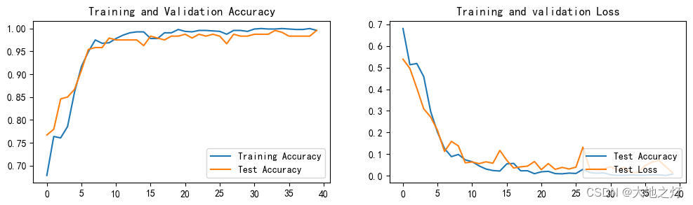
8. 结果可视化
epochs_range = range(epochs)

plt.figure(figsize = (12,3))

plt.subplot(1,2,1)
plt.plot(epochs_range,train_acc,label = 'Training Accuracy')
plt.plot(epochs_range,test_acc,label = 'Test Accuracy')
plt.legend(loc = 'lower right')
plt.title('Training and Validation Accuracy')

plt.subplot(1,2,2)
plt.plot(epochs_range,train_loss,label = 'Test Accuracy')
plt.plot(epochs_range,test_loss,label = 'Test Loss')
plt.legend(loc = 'lower right')
plt.title('Training and validation Loss')
plt.show()

9. 模型的保存
# 自定义模型保存
# torch.save(model.'coffee_bean_rec_model.pth') # 保存整个模型

# 自定义模型加载
# model2 = torch.load('coffee_bean_rec_model.pth')
# model2 = model2.to(device) # 理论上在哪里保存模型,加载模型也会优先在哪里,指定一下确保不会出错
# # vgg16官方模型参数保存
# # 状态字典保存
# torch.save(model.state_dict(),'coffee_bean_rec_model_state_dict.pth') # 仅保存状态字典

# # 加载状态字典到模型
# best_model = vgg16(pretrained = True).to(device) # 定义官方vgg16模型用来加载参数

# for param in best_model.parameters():
#     param.requires_grad = False # 冻结模型参数,这样子在训练的时候只训练最后一层的参数

# best_model.classifier._modules['6'] = nn.Linear(4096,len(classNames)) # 修改vgg16模型中最后一层全连接层,输出目标类别个数
# # best_model = vgg16().to(device) # 重新定义一个模型用来加载参数
# best_model.load_state_dict(torch.load('coffee_bean_rec_model_state_dict.pth')) # 加载状态字典到模型
# 自定义模型保存
# 状态字典保存
torch.save(model.state_dict(),'face_rec_model_state_dict.pth') # 仅保存状态字典

# 加载状态字典到模型
best_model = vgg16().to(device) # 定义官方vgg16模型用来加载参数

best_model.load_state_dict(torch.load('face_rec_model_state_dict.pth')) # 加载状态字典到模型
<All keys matched successfully>
10. 使用训练好的模型进行预测
# 指定路径图片预测
from PIL import Image
import torchvision.transforms as transforms

classes = list(total_data.class_to_idx) # classes = list(total_data.class_to_idx)

def predict_one_image(image_path,model,transform,classes):

    test_img = Image.open(image_path).convert('RGB')
    # plt.imshow(test_img) # 展示待预测的图片

    test_img = transform(test_img)
    img = test_img.to(device).unsqueeze(0)

    model.eval()
    output = model(img)
    print(output) # 观察模型预测结果的输出数据

    _,pred = torch.max(output,1)
    pred_class = classes[pred]
    print(f'预测结果是:{pred_class}')
# 预测训练集中的某张照片
predict_one_image(image_path='./data/coffee_bean_recognize/Light/light (1).png',
                 model = model,
                 transform = test_transforms,
                 classes = classes
                 )
tensor([[-31.8651,   8.0218,  20.2537,  -1.1075]], device='cuda:0',
       grad_fn=<AddmmBackward0>)
预测结果是:Light
11. 不同参数模型预测效果测试与记录-自定义模型(待完善)
固定学习率
动态学习率 + Adam
1e-4 测试集准确率99.6%
 Epoch: 1,Train_acc:67.8%,Train_loss:0.680,Test_acc:76.7%,Test_loss:0.539,Lr:7.79E-05
    Epoch: 2,Train_acc:76.4%,Train_loss:0.513,Test_acc:77.9%,Test_loss:0.496,Lr:7.79E-05
    Epoch: 3,Train_acc:76.0%,Train_loss:0.519,Test_acc:84.6%,Test_loss:0.405,Lr:7.16E-05
    Epoch: 4,Train_acc:78.5%,Train_loss:0.458,Test_acc:85.0%,Test_loss:0.309,Lr:7.16E-05
    Epoch: 5,Train_acc:86.0%,Train_loss:0.297,Test_acc:86.7%,Test_loss:0.272,Lr:6.59E-05
    Epoch: 6,Train_acc:91.7%,Train_loss:0.200,Test_acc:90.8%,Test_loss:0.209,Lr:6.59E-05
    Epoch: 7,Train_acc:94.9%,Train_loss:0.126,Test_acc:95.4%,Test_loss:0.112,Lr:6.06E-05
    Epoch: 8,Train_acc:97.5%,Train_loss:0.089,Test_acc:95.8%,Test_loss:0.159,Lr:6.06E-05
    Epoch: 9,Train_acc:96.8%,Train_loss:0.099,Test_acc:95.8%,Test_loss:0.138,Lr:5.58E-05
    Epoch:10,Train_acc:96.9%,Train_loss:0.074,Test_acc:97.9%,Test_loss:0.060,Lr:5.58E-05
    Epoch:11,Train_acc:97.8%,Train_loss:0.065,Test_acc:97.5%,Test_loss:0.064,Lr:5.13E-05
    Epoch:12,Train_acc:98.5%,Train_loss:0.046,Test_acc:97.5%,Test_loss:0.056,Lr:5.13E-05
    Epoch:13,Train_acc:99.1%,Train_loss:0.031,Test_acc:97.5%,Test_loss:0.065,Lr:4.72E-05
    Epoch:14,Train_acc:99.3%,Train_loss:0.024,Test_acc:97.5%,Test_loss:0.058,Lr:4.72E-05
    Epoch:15,Train_acc:99.3%,Train_loss:0.022,Test_acc:96.2%,Test_loss:0.117,Lr:4.34E-05
    Epoch:16,Train_acc:97.8%,Train_loss:0.055,Test_acc:98.3%,Test_loss:0.071,Lr:4.34E-05
    Epoch:17,Train_acc:97.8%,Train_loss:0.057,Test_acc:97.9%,Test_loss:0.036,Lr:4.00E-05
    Epoch:18,Train_acc:99.1%,Train_loss:0.023,Test_acc:97.5%,Test_loss:0.041,Lr:4.00E-05
    Epoch:19,Train_acc:99.1%,Train_loss:0.023,Test_acc:98.3%,Test_loss:0.045,Lr:3.68E-05
    Epoch:20,Train_acc:99.8%,Train_loss:0.010,Test_acc:98.3%,Test_loss:0.066,Lr:3.68E-05
    Epoch:21,Train_acc:99.4%,Train_loss:0.018,Test_acc:98.8%,Test_loss:0.028,Lr:3.38E-05
    Epoch:22,Train_acc:99.3%,Train_loss:0.021,Test_acc:97.9%,Test_loss:0.056,Lr:3.38E-05
    Epoch:23,Train_acc:99.6%,Train_loss:0.010,Test_acc:98.8%,Test_loss:0.030,Lr:3.11E-05
    Epoch:24,Train_acc:99.6%,Train_loss:0.009,Test_acc:98.3%,Test_loss:0.039,Lr:3.11E-05
    Epoch:25,Train_acc:99.5%,Train_loss:0.012,Test_acc:98.8%,Test_loss:0.031,Lr:2.86E-05
    Epoch:26,Train_acc:99.4%,Train_loss:0.011,Test_acc:98.3%,Test_loss:0.040,Lr:2.86E-05
    Epoch:27,Train_acc:98.8%,Train_loss:0.030,Test_acc:96.7%,Test_loss:0.132,Lr:2.63E-05
    Epoch:28,Train_acc:99.6%,Train_loss:0.015,Test_acc:98.8%,Test_loss:0.031,Lr:2.63E-05
    Epoch:29,Train_acc:99.6%,Train_loss:0.012,Test_acc:98.3%,Test_loss:0.031,Lr:2.42E-05
    Epoch:30,Train_acc:99.4%,Train_loss:0.014,Test_acc:98.3%,Test_loss:0.032,Lr:2.42E-05
    Epoch:31,Train_acc:99.9%,Train_loss:0.004,Test_acc:98.8%,Test_loss:0.042,Lr:2.23E-05
    Epoch:32,Train_acc:100.0%,Train_loss:0.002,Test_acc:98.8%,Test_loss:0.027,Lr:2.23E-05
    Epoch:33,Train_acc:99.9%,Train_loss:0.003,Test_acc:98.8%,Test_loss:0.038,Lr:2.05E-05
    Epoch:34,Train_acc:99.9%,Train_loss:0.004,Test_acc:99.6%,Test_loss:0.014,Lr:2.05E-05
    Epoch:35,Train_acc:100.0%,Train_loss:0.003,Test_acc:99.2%,Test_loss:0.017,Lr:1.89E-05
    Epoch:36,Train_acc:99.9%,Train_loss:0.003,Test_acc:98.3%,Test_loss:0.047,Lr:1.89E-05
    Epoch:37,Train_acc:99.8%,Train_loss:0.004,Test_acc:98.3%,Test_loss:0.063,Lr:1.74E-05
    Epoch:38,Train_acc:99.8%,Train_loss:0.004,Test_acc:98.3%,Test_loss:0.071,Lr:1.74E-05
    Epoch:39,Train_acc:100.0%,Train_loss:0.002,Test_acc:98.3%,Test_loss:0.042,Lr:1.60E-05
    Epoch:40,Train_acc:99.6%,Train_loss:0.008,Test_acc:99.6%,Test_loss:0.014,Lr:1.60E-05
    Done